
Training in ABR
How to Measure Residual Noise
Description
In evoked potential testing, there are various ways to measure residual noise. But which one should you use?
The fully objective and perhaps easiest method is to use the automated residual noise calculator. This feature analyses the sweep-to-sweep variability of the measured and provides a numerical and graphical display of the residual noise. The lower the variance, the more “stable” the averaged waveform becomes.

Here is an example of the graphical and numerical display. The y-axis shows residual noise (0-200 nV), and the x-axis shows number of sweeps (0-8000). A target value of 40 nV is shown by the arrow.
As the number of sweeps increases the variability decreases (more noise is averaged away), showing a curve that decreases rapidly, but then begins to asymptote. This is perfectly normal and the reason for the asymptote is because the remaining noise in an average trace decreases as a function of the square root of the number of trials.
This popular statistical method to evaluate noise is available for the most commonly used evoked potential application – threshold estimation in infants using the Auditory Brainstem Response.
There are other methods also in common use, and could be used during ABR measures but would be relied upon in applications where the automated residual noise calculator is not available, such as the Auditory Middle Latency Response, the Auditory Late Response and Neuro Latency/Rate exams (i.e ABR for differential diagnosis of retrocochlear pathology).
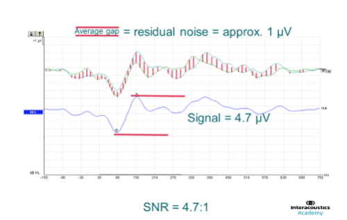
One approach is the “average gap” method, demonstrated below for an N1-P2 complex of the Auditory Late Response.
The lower (blue) trace is an average response of 50 presentations of a 2 kHz toneburst signal; 25 condensation sweeps and 25 rarefaction. These two sub-averages are shown above (A+B curves), with their baselines overlaid. If the noise was zero and these two sub-averages contained the evoked potential only (a hypothetical scenario) then they would overlay perfectly. Any differences between them therefore represents the residual noise. The “average gap” method involves estimating (“by eye”) the difference between the trace by observing the gaps between the trace. The average gap of these A+B curves is shaded for illustration. It is a semi-objective approach since the results are dependent on the interpretation of the observer, although they are based on objectively obtained data.
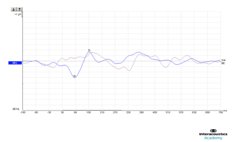
A related method is via the differential (A-B) curve. This subtraction curve will be smaller amplitude (a “flat” trace) when the noise is low and greater in amplitude (a “wavy” trace) when the noise is high. The amplitude of the waveform (e.g. how much it deviates from the baseline) thus gives an objective indication of the residual noise. For example, below is the same data as the previous example but instead of the A and B curves displayed overlaid, the differential curve (A-B) is displayed overlaid onto the average trace. It may be noticed that where the “gap” is large in the previous example, the differential curve deviates far from the baseline whereas when the “gap” is small, the differential curve remains close to the baseline.
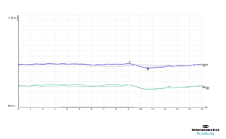
In the final example, below, we see an ABR measured in an infant at 40 dB nHL using the CE-Chirp stimulus in the left ear. The child has a mild hearing loss and the response here is close to threshold. However, a clear wave V is nonetheless present, as demonstrated by the waveform markers showing a faint but clear wave V; the data have an Fmp value of 11.05.
Crucially the residual noise is low with an automated indication of 7nV, very little gap between A+B curves and a “flat” differential curve.
Related course
Presenter
